Generating simulated data#
While fitting a model can be accomplished by evaluating the log likelihood of the data (see Fitting a model), to interpret the behavior of a model with a given set of parameters it’s important to generate simulated data. These data can then be analyzed the same way as real data.
Loading data to simulate#
First, we need an experiment to run. This is specified using psifr DataFrame format. We’ll use data from a sample experiment. Only the study trials are needed in this case. They’ll specify the order in which items are presented in each list during the simulation.
In [1]: from cymr import fit, cmr

In [2]: from psifr import fr

In [3]: data = fit.sample_data('Morton2013_mixed')

In [4]: items = (data
   ...:     .query('trial_type == "study"')
   ...:     .groupby('item_index')
   ...:     .first()['item']
   ...:     .to_numpy()
   ...: )
   ...:

In [5]: data = fr.filter_data(data, subjects=1)

In [6]: fr.filter_data(data, trial_type='study')
Out[6]:
      subject  list  position  ... response response_time  list_category
0           1     2         1  ...      3.0         1.255          mixed
1           1     2         2  ...      3.0         1.040          mixed
2           1     2         3  ...      2.0         1.164          mixed
3           1     2         4  ...      2.0         0.829          mixed
4           1     2         5  ...      3.0         0.872          mixed
...       ...   ...       ...  ...      ...           ...            ...
1062        1    48        20  ...      3.0         0.641          mixed
1063        1    48        21  ...      3.0         0.997          mixed
1064        1    48        22  ...      2.0         0.589          mixed
1065        1    48        23  ...      3.0         0.733          mixed
1066        1    48        24  ...      3.0         0.495          mixed

[720 rows x 12 columns]
Note
It’s also possible to use columns of the DataFrame to set dynamic parameter values that vary over trial. For example, if some lists have a distraction task, you could have context integration rate vary with the amount of distraction. See dynamic parameter methods in Parameters.
Setting parameters#
Next, we define parameters for the simulation. Often these will be
taken from a parameter fit (see Fitting a model). Here, we’ll
just define the parameters we want directly. We also need to create
a CMRParameters object to define how the model
patterns are used.
In [7]: param = {
   ...:     'B_enc': 0.6,
   ...:     'B_start': 0.3,
   ...:     'B_rec': 0.8,
   ...:     'Afc': 0,
   ...:     'Dfc': 0.85,
   ...:     'Acf': 1,
   ...:     'Dcf': 0.85,
   ...:     'Aff': 0,
   ...:     'Dff': 1,
   ...:     'Lfc': 0.15,
   ...:     'Lcf': 0.15,
   ...:     'P1': 0.8,
   ...:     'P2': 1,
   ...:     'T': 0.1,
   ...:     'X1': 0.001,
   ...:     'X2': 0.35
   ...: }
   ...:

In [8]: patterns = {'items': items, 'vector': {'loc': np.eye(768)}}

In [9]: param_def = cmr.CMRParameters()

In [10]: param_def.set_sublayers(f=['task'], c=['task'])

In [11]: weights = {(('task', 'item'), ('task', 'item')): 'loc'}

In [12]: param_def.set_weights('fc', weights)

In [13]: param_def.set_weights('cf', weights)
Running a simulation#
We can then use the data, which define the items to study and recall on each list, with the parameters and patterns, to general simulated data using the CMR model. We’ll repeat the simulation five times to get a stable estimate of the model’s behavior in this task.
In [14]: model = cmr.CMR()

In [15]: sim = model.generate(data, param, param_def=param_def, patterns=patterns, n_rep=5)
Analying simulated data#
We can then use the Psifr package to score and analyze the simulated data just as we would real data. First, we score the data to prepare it for analysis. This generates a new DataFrame that merges study and recall events for each list:
In [16]: sim_data = fr.merge_free_recall(sim)

In [17]: sim_data
Out[17]:
      subject  list                   item  ...  intrusion  prior_list  prior_input
18          1     2              SEAN PENN  ...      False         NaN          NaN
1           1     2         AUDREY HEPBURN  ...      False         NaN          NaN
19          1     2  ST PATRICKS CATHEDRAL  ...      False         NaN          NaN
15          1     2          LES INVALIDES  ...      False         NaN          NaN
8           1     2   GREAT ZIMBABWE RUINS  ...      False         NaN          NaN
...       ...   ...                    ...  ...        ...         ...          ...
3580        1   240            CHE GUEVARA  ...      False         NaN          NaN
3591        1   240             OAHU BEACH  ...      False         NaN          NaN
3585        1   240           GATEWAY ARCH  ...      False         NaN          NaN
3598        1   240            WHITE HOUSE  ...      False         NaN          NaN
3599        1   240       WRIGLEY BUILDING  ...      False         NaN          NaN

[3600 rows x 11 columns]
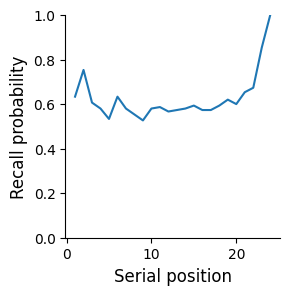
Next, we can plot recall as a function of serial position:
In [18]: recall = fr.spc(sim_data)

In [19]: g = fr.plot_spc(recall)
We can also analyze the order in which items are recalled by calculating conditional response probability as a function of lag:
In [20]: crp = fr.lag_crp(sim_data)

In [21]: g = fr.plot_lag_crp(crp)
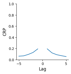
Peaks at short lags (e.g., -1, +1) indicate a tendency for items in nearby serial positions to be recalled successively.
See psifr.fr for more analyses that you can run using Psifr.